From English to Español: Building a Transformer for Language Translation

Hi everyone! Today, we're going on an exciting journey into the world of Artificial Intelligence. We'll be rolling up our sleeves and building our very own translator, a model that can take an English sentence and magically turn it into Spanish. Our secret weapon? The revolutionary "Attention Is All You Need" paper and its star, the Transformer model.

The Transformer: A Game-Changer in the World of NLP

Picture this: it's 2017, and the world of Natural Language Processing (NLP) is about to have its "aha!" moment. A paper titled Attention Is All You Need is published, and it introduces a groundbreaking model called the Transformer. Before the Transformer, models processed sentences word by word in a sequence, like reading a book one word at a time. This could be slow and sometimes the model would forget the beginning of a long sentence by the time it reached the end.

The Transformer changed the game by being able to look at all the words in a sentence at once, weighing their importance. This new approach, built on a clever mechanism called "attention," paved the way for the powerful language models we know and love today, like BERT and GPT.

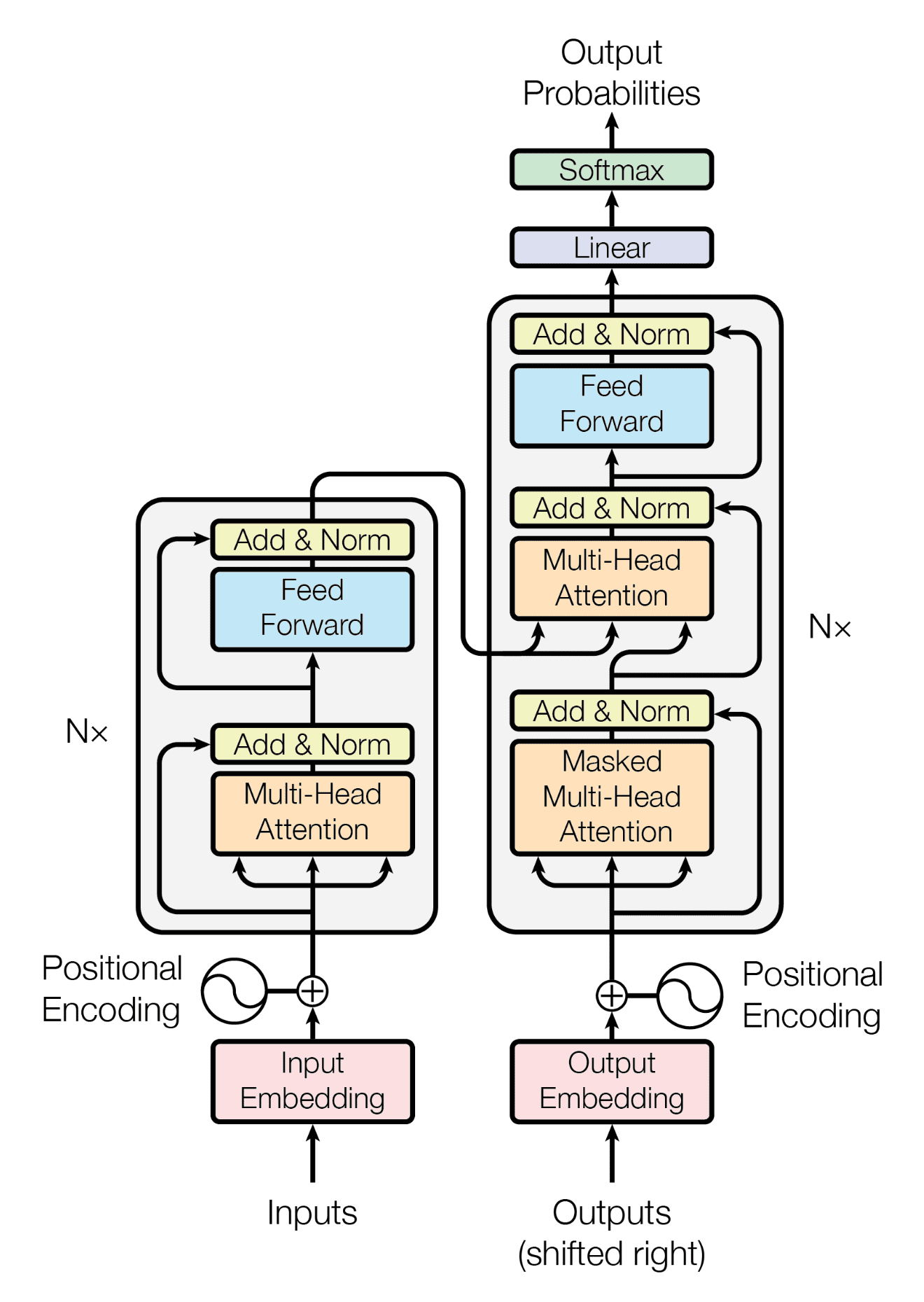
At its heart, the Transformer has two main parts:

• The Encoder: Think of the encoder as a super-smart summarizer. It reads the input sentence (in our case, English) and condenses all its meaning and context into a rich, numerical representation.
• The Decoder: The decoder is like a creative writer. It takes the summary from the encoder and, word by word, writes out the translated sentence in the target language (Spanish).

But what makes the Transformer so special is its attention mechanism. Imagine you're translating the sentence, "The cat sat on the mat." When you're figuring out the Spanish word for "sat," the attention mechanism helps the model pay extra attention to "cat" because who is doing the sitting is very important. This is done through:

• Self-attention: This allows the model to understand the relationships between words in the same sentence. For example, in "The bank of the river," self-attention helps the model understand that "bank" is related to "river" and not a financial institution.
• Multi-head attention: This is like having several people read the same sentence, each focusing on different things. One person might focus on the grammar, another on the meaning, and a third on the nuances. The model then combines all these perspectives for a much richer understanding.

What's a Sequence-to-Sequence (Seq2Seq) Model Anyway?

Before we dive into the code, let's quickly understand the big picture: the Sequence-to-Sequence (Seq2Seq) model. As the name suggests, it's a model designed to convert one sequence into another. Think of it like a magical machine that takes in a string of beads of one color (our English sentence) and outputs a string of beads of another color (the Spanish translation).

• Encoder: This part of the machine scans the entire input sequence and creates a "thought vector" or "context vector" – a numerical summary that captures the essence of the input.
• Decoder: The decoder then takes this "thought vector" and begins generating the output sequence, one element at a time, until the full translation is complete.

We train this model by showing it thousands of examples of English sentences and their corresponding Spanish translations, and over time, it learns the patterns and rules of both languages to become a proficient translator.

Let's Build Our Translator: The Code

Importing Libraries

First things first, we need to gather our tools. We'll be using several Python libraries, including:

• numpy and pandas for handling our data.
• matplotlib for visualizing our data.
• tensorflow and keras for building and training our neural network.
• The Hugging Face tokenizers library for fast, byte-pair encoding tokenization.

import os
import itertools
import numpy as np
import pandas as pd
import tensorflow as tf
from tensorflow.keras.models import Model, Sequential
from tensorflow.keras.layers import Dense, Dropout, Embedding, Input, MultiHeadAttention, LayerNormalization, Layer
from tensorflow.keras.optimizers import Adam
from tensorflow.keras.callbacks import EarlyStopping, ModelCheckpoint
from sklearn.model_selection import train_test_split
import matplotlib.pyplot as plt
from tokenizers import Tokenizer, models, trainers, pre_tokenizers, normalizers

print("GPU is available" if tf.config.list_physical_devices('GPU') else "NOT AVAILABLE")

strategy = tf.distribute.MirroredStrategy()
print(f"Number of GPUs being used: {strategy.num_replicas_in_sync}")

The Blueprint: Our Configuration

Before we touch the data, let's define a single Config class that will hold every hyperparameter we use throughout the project (vocab size, sequence length, file paths, etc.). Keeping all settings in one place makes the pipeline much easier to tune later.

class Config:
    MIX_VOCAB_SIZE = 16000
    EMBED_DIM = 512
    FF_DIM = 1024
    NUM_HEADS = 8

    NUM_ENCODER_LAYERS = 6
    NUM_DECODER_LAYERS = 6
    DROPOUT_RATE = 0.1
    MAX_LENGTH = 96
    BATCH_SIZE = 128
    BUFFER_SIZE = 20000
    EPOCHS = 50
    WARMUP_STEPS = 4000

    CSV_PATH = os.path.join("/dataset_path", "data.csv")

    DATA_DIR = "/working/"
    SP_DIR = os.path.join(DATA_DIR, "sp_data")
    BPE_MODEL_PREFIX = os.path.join(DATA_DIR, "bpe_multi")
    TF_RECORD_TRAIN = os.path.join(DATA_DIR, "train.tfrecord")
    TF_RECORD_VAL = os.path.join(DATA_DIR, "val.tfrecord")

    IS_TRAINING = True

config = Config()

These numbers follow the base Transformer from the paper, 6 encoder + 6 decoder layers, 8 attention heads, and d_model = 512. Dropout is set to 0.1, the value the paper uses for the base model.

Getting Our Data Ready

Download Dataset

This dataset is a CSV file of English and Spanish sentence pairs. We'll load it, drop any rows with missing values, and reset the index so downstream batching stays clean.

def clean_dataset(df):
    print("Initial shape of dataset: ", df.shape)
    df = df.dropna()
    df = df.reset_index(drop=True)
    print("Dataset cleaned. Shape: ", df.shape)
    return df

dataset = pd.read_csv(config.CSV_PATH)
dataset = clean_dataset(dataset)

A quick visualization helps us understand sentence lengths in tokens, so we can later pick a sensible MAX_LENGTH.

def visualize_data(df):
    eng_length = [len(str(s).split()) for s in df["english"].dropna()]
    esp_length = [len(str(s).split()) for s in df["spanish"].dropna()]

    plt.figure(figsize=(10, 6))
    plt.hist(eng_length, label="eng", color="red", alpha=0.33, bins=50)
    plt.hist(esp_length, label="esp", color="blue", alpha=0.33, bins=50)
    plt.yscale("log")
    plt.legend()
    plt.title("Examples count vs Token length")
    plt.xlabel("Token Length")
    plt.ylabel("Count (Log Scale)")
    plt.show()

visualize_data(dataset)

Turning Words into Numbers: Tokenization

Computers don't understand words, they understand numbers. So, we need to convert our sentences into a numerical format. This process is called tokenization. We'll be using a clever technique called Byte-Pair Encoding (BPE) via the Hugging Face tokenizers library, which is significantly faster than the older Python-based options.

Think of BPE like this: instead of just breaking a sentence into words, it can also break words down into smaller, common sub-words. This is super helpful for handling rare or new words. For example, if our model has seen "eating" and "running," BPE might break the new word "jumping" into "jump" and "ing," allowing the model to guess its meaning.

Since English and Spanish share the Latin alphabet and many word roots, we train a single tokenizer on both languages at once. This is more efficient and lets the model exploit cross-lingual overlap. We also stack a few preprocessing steps:

• Normalizer: NFC (canonical composition) ensures visually-identical accented characters share the same byte representation, then Lowercase collapses casing so "Hello" and "hello" don't take up two slots in the vocabulary. We do not strip accents as that would collapse distinct Spanish words like año/ano or sí/si into the same token.
• Pre-tokenizer: Whitespace splits on whitespace, and Digits(individual_digits=True) splits each digit into its own token so numbers don't blow up the vocabulary.
• Special tokens: <pad>, <unk>, <bos>, <eos> are reserved at the start of the vocabulary.

def train_bpe(df):
    """Train BPE on lowercased English+Spanish so vocab is not split across cases."""
    if os.path.exists(config.BPE_MODEL_PREFIX + ".json"):
        return Tokenizer.from_file(config.BPE_MODEL_PREFIX + ".json")

    print("Training BPE model on lowercased corpus...")
    combined_iterator = itertools.chain(
        (s.lower() for s in df['english'].astype(str)),
        (s.lower() for s in df['spanish'].astype(str)),
    )
    bpe_tokeniser = Tokenizer(models.BPE(unk_token="<unk>"))
    bpe_tokeniser.normalizer = normalizers.Sequence([
        normalizers.NFC(),
        normalizers.Lowercase(),
    ])
    bpe_tokeniser.pre_tokenizer = pre_tokenizers.Sequence([
        pre_tokenizers.Whitespace(),
        pre_tokenizers.Digits(individual_digits=True),
    ])
    bpe_trainer = trainers.BpeTrainer(
        vocab_size=config.MIX_VOCAB_SIZE,
        special_tokens=["<pad>", "<unk>", "<bos>", "<eos>"],
        show_progress=True,
    )
    bpe_tokeniser.train_from_iterator(combined_iterator, trainer=bpe_trainer)
    bpe_tokeniser.save(config.BPE_MODEL_PREFIX + ".json")
    return bpe_tokeniser

bpe_tok = train_bpe(dataset)
print("Sample tokens:", bpe_tok.encode("Hello World").tokens)
print("Sample with specials:", bpe_tok.encode("<bos> hola mundo <eos>").ids)

We've set our vocabulary size to 16,000 sub-words shared across both languages. The special tokens are reserved up front, which means <pad> is always 0, <unk> is 1, <bos> is 2, and <eos> is 3.

Preparing the Data for Training

Now we'll split the cleaned DataFrame into a training set (for teaching the model) and a validation set (for checking its progress).

train_df, valid_df = train_test_split(dataset, test_size=0.2, random_state=42)
print(train_df.shape, valid_df.shape)

Next we tokenize both splits. A few important details: we lowercase the source/target text, we wrap each target sentence with <bos> and <eos> as plain text (so the BPE tokenizer turns them into the corresponding special-token IDs in a single pass), and we use the tokenizer's encode_batch method to processes thousands of sentences at once and is dramatically faster than encoding them one by one. Finally, we filter out any pair whose source exceeds MAX_LENGTH or whose target exceeds MAX_LENGTH + 1 (we allow one extra slot because of the <bos>/<eos> wrap).

def tokenize_dataset(df, bpe_tokeniser):
    df_es = df[["english", "spanish"]].dropna().copy()
    df_es["source"] = df_es["english"].str.lower()
    df_es["target"] = df_es["spanish"].str.lower()

    final_df = pd.concat([df_es[["source", "target"]]], ignore_index=True)

    source_texts = final_df["source"].tolist()
    target_texts = ["<bos> " + t + " <eos>" for t in final_df["target"].tolist()]

    source_encodings = bpe_tokeniser.encode_batch(source_texts)
    target_encodings = bpe_tokeniser.encode_batch(target_texts)

    final_df["source_ids"] = [e.ids for e in source_encodings]
    final_df["target_ids"] = [e.ids for e in target_encodings]
    final_df["src_len"] = final_df["source_ids"].map(len)
    final_df["tgt_len"] = final_df["target_ids"].map(len)

    mask = (final_df["src_len"] <= config.MAX_LENGTH) & \
           (final_df["tgt_len"] <= config.MAX_LENGTH + 1)

    filtered_df = final_df.loc[mask, ["source_ids", "target_ids"]].rename(
        columns={"source_ids": "source", "target_ids": "target"}
    ).reset_index(drop=True)

    return filtered_df

train_df = tokenize_dataset(train_df, bpe_tok)
valid_df = tokenize_dataset(valid_df, bpe_tok)

Persisting the Tokenized Data: TFRecords

For each English sentence, the decoder needs two versions of the matching Spanish sentence during training:

1. The Spanish sentence starting with <bos> becomes the decoder input ("Okay, start translating!").
2. The Spanish sentence ending with <eos> becomes the target output (our ground truth).

So we're going from:

• English: "I am learning Deep Neural Networks"
• Spanish: "Yo estoy aprendiendo redes neuronales profundas"

To:

• Encoder Input: [I, am, learning, Deep, Neural, Networks]
• Decoder Input: [<bos>, Yo, estoy, aprendiendo, redes, neuronales, profundas]
• Decoder Output: [Yo, estoy, aprendiendo, redes, neuronales, profundas, <eos>]

This setup allows the model to learn to predict the next word based on the English sentence plus what it has already generated.

Teacher Forcing Method

The method we are implementing is known as Teacher Forcing. At every timestep we provide the decoder with two inputs: the encoded source sentence and the correct target token from the previous timestep (not whatever the model itself produced). This way the model learns to predict the next word given a clean history, instead of compounding its own mistakes.

Time Step	Encoder Input	Decoder Input	Target Output
1	I	<bos>	Yo
2	am	Yo	estoy
3	learning	estoy	aprendiendo
4	Deep	aprendiendo	redes
5	Neural	redes	neuronales
6	Networks	neuronales	profundas
7		profundas	<eos>

Rather than keeping every tokenized sentence in RAM, we serialize the tokenized splits to TFRecord files. TFRecords are TensorFlow's native binary format which are small, fast to read, and they integrate cleanly with the tf.data API for streaming. We then read them back lazily, and the split_target helper produces the (source, target_in, target_out) triple by shifting the target sequence.

def serialize_example(src, trg):
    feature = {
        "source": tf.train.Feature(int64_list=tf.train.Int64List(value=src)),
        "target": tf.train.Feature(int64_list=tf.train.Int64List(value=trg)),
    }
    return tf.train.Example(features=tf.train.Features(feature=feature)).SerializeToString()

def parse_fn(example):
    feature_description = {
        "source": tf.io.VarLenFeature(tf.int64),
        "target": tf.io.VarLenFeature(tf.int64),
    }
    example = tf.io.parse_single_example(example, feature_description)
    src = tf.sparse.to_dense(example["source"])
    trg = tf.sparse.to_dense(example["target"])
    return src, trg

def create_tfrecords(dataset, filename):
    with tf.io.TFRecordWriter(filename) as writer:
        for s, t in dataset.itertuples(index=False):
            writer.write(serialize_example(s, t))

def split_target(src, trg):
    return src, trg[:-1], trg[1:]

create_tfrecords(train_df, config.TF_RECORD_TRAIN)
create_tfrecords(valid_df, config.TF_RECORD_VAL)

train_dataset_raw = (
    tf.data.TFRecordDataset(config.TF_RECORD_TRAIN)
    .map(parse_fn, num_parallel_calls=tf.data.AUTOTUNE)
    .map(split_target, num_parallel_calls=tf.data.AUTOTUNE)
)

valid_dataset_raw = (
    tf.data.TFRecordDataset(config.TF_RECORD_VAL)
    .map(parse_fn, num_parallel_calls=tf.data.AUTOTUNE)
    .map(split_target, num_parallel_calls=tf.data.AUTOTUNE)
)

Token Bucketing and Padding

Finally, we organize our data into batches grouped by length. Bucketing is like sorting laundry by color before washing, so in our case it is the putting sentences of similar lengths in the same batch means we don't waste compute on padding.

But there's an extra twist: instead of using a fixed BATCH_SIZE for every bucket, we allocate a fixed token budget per batch (TOKENS_PER_BATCH = 4096, scaled up by the number of GPUs in the MirroredStrategy). Short sentences pack tightly (~256+ per batch for length ≤ 16), and long ones pack sparsely (~40 per batch for length ≤ 100). This way every batch does roughly the same amount of work on the GPU, which keeps training throughput steady.

Why bucketing and padding

Sentences in our dataset aren't all the same length, so we add padding tokens (<pad> = id 0) to align them within a batch. If we naively padded every sentence in the dataset up to the longest one, we'd waste enormous compute on padding tokens and the model could even pick up bad habits from the padded positions.

Bucketing solves this: each batch only pads up to the longest sentence in that batch, which is close to the bucket boundary. Combined with a token-based batch size, both short-sentence batches and long-sentence batches stay GPU-friendly.

num_replicas = strategy.num_replicas_in_sync

BUFFER_SIZE = 10000
TOKENS_PER_BATCH = 4096
TOKENS_PER_BATCH = TOKENS_PER_BATCH * num_replicas

def element_length_func(inputs, targets):
    return tf.shape(inputs["encoder_inputs"])[0]

def format_dataset(src, trg_in, trg_out):
    return ({"encoder_inputs": src, "decoder_inputs": trg_in}, trg_out)

bucket_boundaries = [16, 32, 64, 96]
bucket_batch_sizes = [int(TOKENS_PER_BATCH / x) for x in bucket_boundaries]
bucket_batch_sizes.append(int(TOKENS_PER_BATCH / 100))
print(f"Bucket batch sizes: {bucket_batch_sizes}")
# On 2 GPUs -> [512, 256, 128, 85, 81]

train_ds = (
    train_dataset_raw
    .map(format_dataset, num_parallel_calls=tf.data.AUTOTUNE)
    .cache()
    .shuffle(BUFFER_SIZE)
    .bucket_by_sequence_length(
        element_length_func=element_length_func,
        bucket_boundaries=bucket_boundaries,
        bucket_batch_sizes=bucket_batch_sizes,
        padding_values=(
            {"encoder_inputs": tf.constant(0, dtype=tf.int64),
             "decoder_inputs": tf.constant(0, dtype=tf.int64)},
            tf.constant(0, dtype=tf.int64)
        ),
        drop_remainder=True,
    )
    .prefetch(tf.data.AUTOTUNE)
)

valid_ds = (
    valid_dataset_raw
    .map(format_dataset, num_parallel_calls=tf.data.AUTOTUNE)
    .bucket_by_sequence_length(
        element_length_func=element_length_func,
        bucket_boundaries=bucket_boundaries,
        bucket_batch_sizes=bucket_batch_sizes,
        padding_values=(
            {"encoder_inputs": tf.constant(0, dtype=tf.int64),
             "decoder_inputs": tf.constant(0, dtype=tf.int64)},
            tf.constant(0, dtype=tf.int64)
        ),
        drop_remainder=True,
    )
    .prefetch(tf.data.AUTOTUNE)
)

print("Data pipelines created successfully using the stable API.")

And there you have it! Our data is now perfectly prepped and ready to be fed into our Transformer model. In the next part, we'll build the model architecture itself and start the training process. Stay tuned!